Available neural network-based models for predicting the oil flow rate (qo) in the Niger Delta are not simplified and are developed from limited data sources. The reproducibility of these models is not feasible as the models’ details are not published. This study developed simplified and reproducible three, five, and six-input variables neural-based models for estimating qo using 283 datasets from 21 wells across fields in the Niger Delta. The neural-based models were developed using maximum-minimum (max.-min.) normalized and clip-normalized datasets. The performances and the generalizability of the developed models with published datasets were determined using some statistical indices: coefficient of determination (R2), mean square error (MSE), root mean square error (RMSE), average relative error (ARE) and average absolute relative error (AARE). The results indicate that the 3-input-based neural models had overall R2, MSE, and RMSE values of 0.9689, 9.6185x10⁻⁴ and 0.0310, respectively, for the max.-min. normalizing method and R2 of 0.9663, MSE of 5.7986x10⁻³ and RMSE of 0.0762 for the clip scaling approach. The 5-input-based models resulted in R2 of 0.9865, MSE of 5.7790×10⁻⁴ and RMSE of 0.0240 for the max.-min. scaling method and R2 of 0.9720, MSE of 3.7243x10⁻³ and RMSE of 0.0610 for the clip scaling approach. Also, the 6-input-based models had R2 of 0.9809, MSE of 8.7520x10⁻⁴ and RMSE of 0.0296 for the max.-min. normalizing approach and R2 of 0.9791, MSE of 3.8859 x 10⁻³ and RMSE of 0.0623 for the clip scaling method. Furthermore, the generality performance of the simplified neural-based models resulted in R2, RMSE, ARE, and AAPRE of 0.9644, 205.78, 0.0248, and 0.1275, respectively, for the 3-input-based neural model and R2 of 0.9264, RMSE of 2089.93, ARE of 0.1656 and AARE of 0.2267 for the 6-input-based neural model. The neural-based models predicted qo were more comparable to the test datasets than some existing correlations, as the predicted qo result was the lowest error indices. Besides, the overall relative importance of the neural-based models’ input variables on qo prediction is S>GLR>Pwh>T/Tsc>γo>BS&W>γg. The simplified neural-based models performed better than some empirical correlations from the assessment indicators. Therefore, the models should apply as tools for oil flow rate prediction in the Niger Delta fields, as the necessary details to implement the models are made visible.
| Published in | Petroleum Science and Engineering (Volume 8, Issue 2) |
| DOI | 10.11648/j.pse.20240802.12 |
| Page(s) | 70-99 |
| Creative Commons |
This is an Open Access article, distributed under the terms of the Creative Commons Attribution 4.0 International License (http://creativecommons.org/licenses/by/4.0/), which permits unrestricted use, distribution and reproduction in any medium or format, provided the original work is properly cited. |
| Copyright |
Copyright © The Author(s), 2024. Published by Science Publishing Group |
Neural Network, Normalization Methods, Simplified Neural-Based Models, Oil Flow Rate, Niger Delta
# | Author(s) | Datasets Source / Points | Artificial Intelligence Approach | Input Variables | Output Variable | Model Performance | Model / Architecture Pitfall |
|---|---|---|---|---|---|---|---|
1 | Berneti and Shahbazian [28] | Source: Iran Oilfield Datasets: 31 oil wells | ANN and ICA Architecture: 2-7-1 | Pwh, T |
| MSE = 0.0123 RMSE = 0.1109 R2 = 0.9703 R = 0.9850 | The models’ structures are simple and applicable for development. |
2 | Mirzaei-Paiaman and Salavati [29] | Source: Iran Oilfield Datasets: 134 | ANN Architecture: 3-4-1 | Pwh, S, GOR |
| AARE = 2.110 ARE = -0.330 R2 = 0.9998 R = 0.9999 | |
3 | Ahmadi et al. [ 50] | Source: Iran Oilfields Datasets: 50 oil wells; 1600 | ANN Architecture: N/A | Pwh, T |
| MSE = 0.0913 RMSE = 0.3022 R2 = 0.9391 R = 0.9691 | Models’ structures are not provided to assess their simplicity and applicability. |
ANN-ICA Architecture: N/A | MSE = 0.0030 RMSE = 0.0551 R2 = 0.9951 R = 0.9976 | ||||||
4 | Al-Khalifa and Al-Marhoun [30] | Source: Middle East fields Datasets: 4031 | ANN Architecture: 6-9-5-8-1 | Pwh, T, S, GOR, |
| MSE = 110.25 RMSE = 10.50 R2 = 0.9860 R = 0.9930 | The model architecture is complex and not applicable. |
5 | Zangl et al. [31] | Source: N/A Datasets: 258 | ANN Architecture: N/A | Pwh, |
| R2 = 0.9308 R = 0.9648 | Models’ structures are not provided to assess their simplicity and applicability. |
6 | Gorjaei et al. [5 1] | Source: Iran Oilfields Datasets: 276 | PSO-LSSVM Architecture: N/A | S, Pwh, GLR |
| AARE = 0.70 R2 = 0.9935 R = 0.9967 | |
7 | Hasanvand and Berneti [5 2] | Source: Iran Oilfields Datasets: 600 | ANN Architecture: 2-7-1 | T, |
| MSE = 0.0094 RMSE = 0.097 R2 = 0.9874 R = 0.9937 | The model architecture is simple and applicable for development. |
8 | Al-Ajmi et al. [32] | Source: N/A Datasets: 174 | ANN Architecture: N/A | Pwh, S, T, GOR, WCT |
| MAPE = 15.15 R2 = 0.890 R = 0.9434 | Model architecture is not provided to assess its simplicity and application. |
9 | Okon and Appah [33] | Source: Niger Delta Oilfields Datasets: 64 | ANN Architecture: 3-6-5-1 | Pwh, S, GLR |
| AARE = 0.1920 R2 = 0.9653 R = 0.9825 | Models’ structures (two hidden layers) could be more complex. |
ANN Architecture: 5-6-6-1 | Pwh, S, GLR, T, BS&W | AARE = 0.1045 R2 = 0.9951 R = 0.9976 | |||||
10 | Baghban et al. [5 3] | Source: Iran Oilfields Datasets: 100 | SVM Architecture: N/A | Pwh, S, GOR |
| R2 = 0.9998 R = 0.9999 | Models’ structures are not provided to assess their simplicity and applicability. |
11 | Buhulaigah et al. [5 4] | Source: Middle East Oilfields Datasets: 174 | ANN Architecture: N/A | Pwh, Le, S, |
| R2 = 0.9140 R = 0.9560 | |
12 | Choubineh et al. [12] | Source: Iran Oilfields Datasets: 113 | ANN-TLBO Architecture: N/A | Pwh, S, GLR, T, |
| AARE = 6.50 ARE = 2.09 R2 = 0.9810 R = 0.9905 | |
13 | Al-Qutami et al. [34] | Source: N/A Datasets: 238 | NN ensemble and ASA Architecture: N/A | T, Pwh, BHP, S |
| MAPE = 4.70 MSE = 0.0034 RMSE = 0.0585 | |
14 | Khan et al. [5 5] | Source: N/A Datasets: 1500 | ANN Architecture: 5-6-1 | Pwh, S, T, |
| AARE = 2.50 R2 = 0.9940 R = 0.9970 | Models’ structures have a single hidden layer that is simple to apply. |
15 | Al-Kadem et al. [35] | Source: N/A Datasets: 1854 | ANN Architecture: 3-10-1 | Pwh, S, GOR |
| AARE = 3.70 R2 = 0.80 R = 0.8944 | |
16 | Ghorbani et al. [5 6] | Source: Iran Oilfields Datasets: 182 | GA Architecture: N/A | Pwh, S, GLR, BS&W |
| AARE = 7.33 ARE = -2.890 R2 = 0.9970 R = 0.9985 | Models’ structures are not provided to assess their simplicity and applicability. |
17 | Khan et al. [36] | Source: Asian Oilfields Datasets: 1400 | ANN Architecture: N/A | S, Pwh, T, |
| AARE = 2.5618 R2 = 0.9934 R = 0.9967 | |
18 | Al-Rumah et al. [5 7] | Source: Existing works Datasets: 1111 | ANN Architecture: 3-39-23-1 | Pwh, S, GLR |
| AARE = 0.2206 R2 = 0.9292 R = 0.9640 | Model architecture is too complex to be applicable |
19 | Marfo and Kporxah [5 8] | Source: Ghana Oilfields Datasets: 1600 | ANN Architecture: 4-2-1 |
|
| MAPE = 3.18 R2 = 0.9966 R = 0.9983 | Model architecture is simple for application. |
20 | Ibrahim et al. [37] | Source: Middle East Oilfields Datasets: 548 wells | SVM Architecture: N/A | Pwh, S, GOR |
| AAPE = 1.40 R2 = 0.930 R = 0.9644 | The AI models’ structures are not visible for assessment. |
RF Architecture: N/A | AAPE = 0.75 R2 = 0.940 R = 0.9695 | ||||||
21 | Okorugbo et al. [38] | Source: Niger Delta Oilfields Datasets: 1595 from 7 fields | ANN Architecture: N/A | Pwh, S, GLR, GOR, |
| AARE = 28.44 APE = 7.64 R2 = 0.8774 R = 0.9367 | Models’ structures are not provided to assess their simplicity and applicability. |
ANN-PSO Architecture: N/A | AARE = 35.83 APE = 12.20 R2 = 0.8318 R = 0.9120 | ||||||
22 | Alarifi [27] | Source: N/A Datasets: 1595 from 7 fields | ANN Architecture: N/A | S, Pwh, T, GLR, GOR, WCT |
| MAPE = 19.33 R2 = 0.8649 R = 0.930 | |
23 | Azim [5 9] | Source: Egypt Oilfields Datasets: 350 from 12 fields | ANN Architecture: 6-10-1 | WHT, GLR, WCT, BHT, H, At |
| MSE = 0.020 RMSE = 0.1414 R2 = 0.9630 R = 0.9813 | Model architecture is a single hidden layer with less complexity for application. |
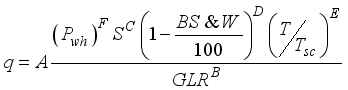
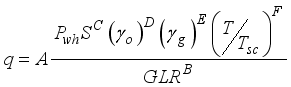
 ), basic sediments and water (BS&W), well-flowing temperature (T), gas gravity (γg), as the input data, and oil flow rate (
  ) as the output datasets. The gathered datasets were as required for Gilbert
 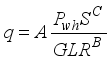 (1)
(1)  (2)
(2)  (3)
(3)  (4)
(4) 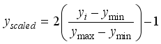 (5)
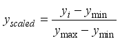
(5)  represents the scaled values for input or output parameters,
  is the values of the not-scaled parameters,
  and
and  denote the minimum and maximum values of the not-scaled parameters, respectively. According to Okon and Ansa
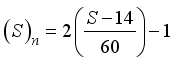
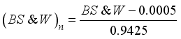
 Parameters | Maximum | Minimum | Range | Average | Std. Dev. |
|---|---|---|---|---|---|
Wellhead Pressure, | 3600.0 | 53.65 | 3546.35 | 977.136 | 831.215 |
Bean (Choke) Size, | 114.0 | 14.0 | 100.0 | 48.532 | 26.285 |
Gas-Liquid Ratio, | 32851.7 | 20.175 | 32831.5 | 2851.31 | 5205.32 |
Oil Gravity, | 0.9433 | 0.643 | 0.3003 | 0.8612 | 0.0564 |
Basic Sediments and Water, | 0.9750 | 0.0005 | 0.9745 | 0.7626 | 0.2104 |
Well Flowing Temperature, | 192.0 | 48.0 | 144.0 | 97.627 | 31.606 |
Gas Gravity, | 0.9399 | 0.5227 | 0.4172 | 0.7410 | 0.0974 |
Oil Flow Rate, | 14417.0 | 183.0 | 14234.0 | 2616.11 | 2933.33 |
Parameters | Maximum | Minimum | Range | Average | Std. Dev. |
|---|---|---|---|---|---|
Wellhead Pressure, | 3300.0 | 95.0 | 3205.0 | 956.318 | 737.64 |
Bean (Choke) Size, | 74.0 | 14.0 | 60.0 | 33.753 | 14.815 |
Gas-Liquid Ratio, | 28597.0 | 29.0 | 28568.0 | 2435.81 | 5025.79 |
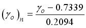
Oil Gravity, | 0.9433 | 0.7339 | 0.2094 | 0.8361 | 0.0443 |
Basic Sediments and Water, | 0.9430 | 0.0005 | 0.9425 | 0.7442 | 0.2053 |
Well Flowing Temperature, | 186.0 | 48.0 | 138.0 | 99.747 | 29.736 |
Gas Gravity, | 0.9399 | 0.5227 | 0.4172 | 0.7410 | 0.0974 |
Oil Flow Rate, | 14417.0 | 183.0 | 14234.0 | 2616.11 | 2933.33 |
 ). The scaled datasets from Equations 4 and 5 were grouped based on Gilbert
  and γg (6-input) for the Choubineh et al.’s model. These scaled data (i.e., inputs and output) were imported from Microsoft Excel to the MATLAB workspace, named accordingly, and saved. Afterward, the nftool environment was active from the command window, and the data files in the workspace moved to the nftool environment for neural network development and training. The neural network training to determine the number of hidden layer neurons was a trial-and-error approach. The networks learned the input and output datasets using the Leverberg-Marquardt algorithm based on the feed-forward back-propagation (FFBP) approach. The network generates the initial weights and biases using its random number generator. Thus, the input datasets, output data, weights, biases, and neurons at the hidden layer are combined to create the network. The outcomes of the network training (70% of the datasets), validation (15% of the datasets) and testing (15% of the datasets), based on the mean square error (MSE) and correlation coefficient (R) values, determine the network performance. For more details on the networks’ stopping criteria and weight adjustment, readers can obtain from published works by Mahmoudi and Mahmoudi
 Hyperparameters | Values |
|---|---|
Training Datasets | 199 (70% of the datasets) |
Validation Datasets | 42 (15% of the datasets) |
Testing Datasets | 42 (15% of the datasets) |
Hidden Layer | 1 |
Hidden Layer Neurons | 5, 6, 8 |
Hidden Layer Activation Function | tansig |
Output Layer Activation Function | purelin |
Learning Algorithm | Levenberg-Marquardt |
Number of Epochs | 1000 |
Rate of Learning | 0.7 |
Architecture Selection | Trial-and-error |
Target Goal MSE | 10-7 |
Minimum Performance Gradient | 10-7 |
 ) data. The observation is because the MSE and R2 values are within acceptable limits for any model/network performance. Therefore, the networks can predict the fields’
  with a 99.0% certainty based on the R2 values obtained. Again, the closeness of the network predicted
  with the actual
  datasets is visible on the diagonal trend of the output (i.e., network predictions) and target (field datasets) for the overall performance, as in Figures 7 to 9. According to Al-Bulushi et al.
 Models | Indices | Maximum-minimum Method | Clip Method | |||||||
|---|---|---|---|---|---|---|---|---|---|---|
Training | Validation | Testing | Overall | Training | Validation | Testing | Overall | |||
i. | 3-input-based model | MSE | 1.3421x10⁻³ | 9.6157x10⁻⁴ | 1.5935x10⁻³ | 9.6158x10⁻⁴ | 5.5103x10⁻³ | 5.7986x10⁻³ | 6.5508x10⁻⁴ | 5.7986x10⁻³ |
R2 | 0.9918 | 0.9950 | 0.9905 | 0.9921 | 0.9929 | 0.9926 | 0.9884 | 0.9915 | ||
ii. | 5-input-based model | MSE | 5.8034x10⁻⁴ | 5.7790x10⁻⁴ | 4.7800x10⁻⁴ | 5.779x10⁻⁴ | 5.1033x10⁻³ | 3.7243x10⁻³ | 4.2300x10⁻³ | 3.7243x10⁻³ |
R2 | 0.9971 | 0.9942 | 0.9932 | 0.9966 | 0.9929 | 0.9922 | 0.9945 | 0.9929 | ||
iii. | 6-input-based model | MSE | 8.2605x10⁻⁴ | 8.7523x10⁻⁴ | 7.2486 x10⁻⁴ | 8.7523x10⁻⁴ | 3.0894 x10⁻³ | 6.9058 x10⁻³ | 2.4769 x10⁻⁴ | 3.8859x10⁻³ |
R2 | 0.9949 | 0.9962 | 0.9955 | 0.9952 | 0.9953 | 0.9923 | 0.9955 | 0.9947 | ||
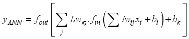 (6)
(6)  is the network predicted output (in normalized form),
  denotes the output neuron activation function (i.e., purelin),
  represents the hidden layer neurons’ weights from the jth neuron to the kth output layer neuron,
  is the transfer function (tansig) at the hidden neuron,
  is the input layer weights from the ith neuron to the jth hidden layer neuron, and
  represents an input variable. Then,
  and
and  represent the hidden and output layers nodes’ biases, respectively. Therefore, based on the established architectures for the neural network-based models for
  prediction, their computation notations are presented in Equations 7 to 9; 3-input-based model:
 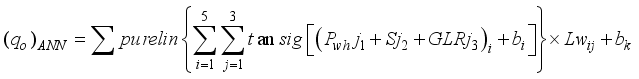 (7)
(7)  (8)
(8)  (9)
(9)  is the neural network predicted oil flow rate in normalized form. The variables
  ,
,  ,
,  ,
,  ,
,  and
and  are the weights of the network inputs:
  ,
,  ,
,  ,
,  ,
,  ,
,  and
and  to the hidden layer neuron;
  represents the hidden layer weights that connect the output layer neuron;
  and
and  are biases at the hidden and output neurons, respectively. Then, purelin and tansig are activation functions at the output and hidden layers’ neurons. The weights and biases of the various neural network-based models for oil flow rate prediction are in Tables 6 to 11.
 Input layer weights | Hidden biases and weights | Output bias | ||||
|---|---|---|---|---|---|---|
| ( | ( | ( |
|
|
|
1 | -0.5385402 | -1.0111643 | -0.3697213 | 1.974864 | -1.1109503 | -0.1585362 |
2 | -1.2660117 | 5.7652163 | 2.0999111 | -3.1918448 | 0.8373804 | |
3 | 0.29895761 | 1.3578018 | -1.9698251 | -2.8393038 | 5.1375123 | |
4 | 0.24131335 | 2.1912495 | -0.5929832 | -2.0673442 | -2.6497395 | |
5 | 1.01553212 | -1.3477269 | 1.15601166 | 3.3939060 | 3.6110957 | |
Input layer weights | Hidden biases and weights | Output bias | ||||
|---|---|---|---|---|---|---|
| ( | ( | ( |
|
|
|
1 | -1.9102399 | 0.1173669 | -0.9406521 | 2.8339813 | 0.16789125 | 1.188847 |
2 | 2.1891470 | -0.4798915 | -3.5388877 | -1.4183450 | 0.38368504 | |
3 | 0.7112502 | 2.47403781 | -3.539615 | -1.3528274 | -0.28206409 | |
4 | -1.0860498 | -0.7007909 | 4.3089994 | 4.66603469 | -2.55714526 | |
5 | 1.6228026 | -2.7474310 | -2.0315176 | -2.3284541 | -0.37376004 | |
Input weights | Hidden biases | Hidden weights | Output bias | |||||
|---|---|---|---|---|---|---|---|---|
| ( | ( | ( | ( | ( |
|
|
|
1 | 3.4900924 | -7.731092 | -6.4360719 | 2.09776475 | 6.6313152 | -11.863917 | -2.3205470 | 0.3472364 |
2 | 3.4423928 | -7.372197 | -6.3975091 | 2.06356456 | 6.4071733 | -11.511381 | 2.3664439 | |
3 | 0.0299627 | 1.7319449 | -0.2676342 | -0.56557378 | -0.4638709 | 1.4411783 | 0.17676961 | |
4 | 0.8098289 | 1.0948423 | -3.4110332 | 0.727664266 | 0.0829497 | -4.0252434 | 1.6790642 | |
5 | -7.188589 | 5.6356843 | 6.7863179 | 7.263317569 | -0.5029194 | -4.1082139 | 4.9673305 | |
6 | -5.888010 | 4.8817139 | 0.50369342 | 6.2700012 | -0.30080753 | -8.6339629 | -5.3101384 | |
Input weights | Hidden biases | Hidden weights | Output bias | |||||
|---|---|---|---|---|---|---|---|---|
| ( | ( | ( | ( | ( |
|
|
|
1 | 0.9010532 | 0.6868277 | -3.3368676 | 0.3989323 | -0.0023792 | -3.695982 | 1.7599079 | 0.662883 |
2 | -0.994761 | 2.1941044 | 0.4255441 | -3.6930451 | 1.69289456 | 3.0435556 | 0.1249966 | |
3 | 2.7616773 | -2.832146 | -2.1586329 | -0.6128486 | 3.78528638 | -2.1373435 | 0.0529069 | |
4 | 0.4204269 | 0.0523971 | -1.1852713 | -0.3920006 | 0.44395427 | -0.655956 | -0.2171184 | |
5 | 1.1663272 | 0.6718416 | -2.0633890 | -0.1329151 | -0.1273617 | 0.2522338 | 0.133396 | |
6 | -0.269904 | -2.297810 | 1.6909864 | 0.3070311 | -1.4469666 | 1.7310819 | -0.0644734 | |
Input weights | Hidden biases | Hidden weights | Output bias | ||||||
|---|---|---|---|---|---|---|---|---|---|
| ( | ( | ( | ( | ( | ( |
|
|
|
1 | 0.047515 | 0.130103 | 0.44245 | -2.030657 | 0.581165 | -0.089446 | 1.970767 | 0.4357025 | 0.235916 |
2 | -1.011681 | 0.891035 | 0.020582 | -1.195120 | -1.019611 | -0.161630 | 1.139384 | 0.0776338 | |
3 | 0.316439 | 0.309080 | -0.488147 | 1.140003 | -0.367717 | 0.6344811 | -0.450963 | 0.3284348 | |
4 | -0.316973 | -0.908201 | 0.045713 | 0.607017 | -1.051208 | -1.110216 | -0.172092 | -0.1304821 | |
5 | 0.632287 | 0.294746 | -0.235050 | -0.862207 | -0.594977 | -0.928184 | 0.637973 | 0.2560455 | |
6 | 0.594650 | 0.439590 | -0.827425 | -1.193106 | 0.6061402 | 0.1739179 | 1.484508 | -0.260832 | |
7 | -0.626795 | 0.869463 | -0.980515 | 0.176416 | -0.468085 | -0.577010 | -1.364878 | -0.036701 | |
8 | -0.560974 | -0.483019 | 1.727690 | -0.821655 | -0.648451 | -0.043607 | 2.329126 | -1.3554218 | |
Input weights | Hidden biases | Hidden weights | Output bias | ||||||
|---|---|---|---|---|---|---|---|---|---|
| ( | ( | ( | ( | ( | ( |
|
|
|
1 | -0.802896 | 1.032175 | 0.523643 | 1.267974 | 0.494186 | -0.555345 | 2.146365 | 0.071464 | -0.65368 |
2 | -0.5326472 | 0.391553 | 0.265645 | -1.635991 | 0.504839 | -0.119175 | -0.794149 | -0.523327 | |
3 | -0.000600 | -0.864577 | 0.055065 | 0.576637 | -0.537443 | -0.721054 | 0.014171 | -0.769143 | |
4 | 0.688203 | 2.37251 | -1.50568 | 2.36764 | 0.877263 | 0.617937 | 0.603996 | -0.068565 | |
5 | 0.523447 | 0.539761 | -0.702578 | 2.091369 | 1.525157 | 0.449091 | -1.461013 | 0.493293 | |
6 | -0.832304 | -0.934466 | 0.977342 | -0.880203 | -0.200528 | 0.809025 | -1.422903 | 0.385712 | |
7 | -1.877361 | -0.722014 | -0.02678 | -0.280917 | -0.139388 | 0.215438 | -1.82908 | -0.136098 | |
8 | 0.233416 | 0.240730 | 0.911708 | -0.095287 | -0.241667 | -1.41470 | 2.185845 | 0.587712 | |
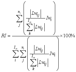 (10)
(10)  is the input layer weights,
  denotes the hidden layer weights to the output neuron,
  and
and  represent the numbers of inputs and hidden layer’s neurons. The outcomes of the RI assessment on the networks’ input variables are in Table 12.
 Model | Scaling method | Input Variables Relative Importance (%) | |||||||
|---|---|---|---|---|---|---|---|---|---|
Pwh | S | GLR | T/Tsc | BS&W | γo | γg | |||
i. | 3-input-based | Max.-min. | 17.40 | 52.80 | 28.80 | NA | NA | NA | NA |
RI ranking | 3rd | 1st | 2nd | NA | NA | NA | NA | ||
Clip | 26.01 | 26.64 | 47.35 | NA | NA | NA | NA | ||
RI ranking | 3rd | 2nd | 1st | NA | NA | NA | NA | ||
ii. | 5-input-based | Max.-min. | 16.68 | 30.07 | 23.56 | 18.00 | 11.69 | NA | NA |
RI ranking | 4th | 1st | 2nd | 3rd | 5th | NA | NA | ||
Clip | 16.68 | 19.51 | 35.06 | 12.93 | 15.82 | NA | NA | ||
RI ranking | 3rd | 2nd | 1st | 5th | 4th | NA | NA | ||
iii. | 6-input-based | Max.-min. | 13.24 | 13.90 | 15.62 | 27.29 | NA | 17.36 | 12.59 |
RI ranking | 5th | 4th | 3rd | 1st | NA | 2nd | 6th | ||
Clip | 16.59 | 19.02 | 12.72 | 23.76 | NA | 12.20 | 15.71 | ||
RI ranking | 3rd | 2nd | 5th | 1st | NA | 6th | 4th | ||
 ,
,  and
and  ) from the input neurons multiply with input weights (
  ,
,  and
and  ), respectively, and are linked to hidden layer neurons;
  ) from the input layer combined with the neuron’s bias (
  ) and the sum (i.e.,
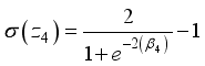
  ) is transformed by the sigmoid function (Equation 11), to the output neuron;
  (11)
(11)  is
is 
 ) multiplied by the hidden neuron weight (
  ) and linked to the output neuron;
  ), thus,
  ;
;  is transformed using the purelin function as the network’s output. Thus, the predicted values are
 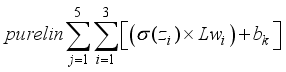 .
.  ,
,  ,
,  ,
,  ,
,  and
and  are in Tables 5 and 6, and they could be applied to other networks (i.e., 5-input-based and 6-input-based) with appropriate adjustments to the network’s variables. The output from the neural network is presented in the normalized form and would require de-normalization to transform the network predictions to a required format (values). Thus, the simplified neural network-based models for oil flow rate prediction are in Equations 12 and 13, based on maximum-minimum and clip scaling approaches;
 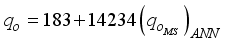 (12)
(12)  (13)
(13)  is the de-normalized oil flow rate,
  and
and  are the predicted oil flow rates (in normalized form) based on the maximum-minimum and the clip scaling methods, respectively, from the neural network. Thus,
  and
and  are expressed in Equations 14 and 15;
  (14)
(14)  (15)
(15)  to
to  in Equations 14 and 15 are expressed as
  ,
,  ,
,  ,
,  and
and  , where
  to
to  are the computations at the hidden layer neurons. For the 3-input-based network with the maximum-minimum scaling method,
  to
to  are expanded as Equations 16 to 20;
  (16)
(16)  (17)
(17)  (18)
(18)  (19)
(19)  (20)
(20)  to
to  for the 3-input-based network with the clip scaling method are expressed as Equations 21 to 25;
  (21)
(21)  (22)
(22)  (23)
(23)  (24)
(24)  (25)
(25)  ,
,  , and
, and  are the normalized input variables (i.e.,
  ,
,  , and
, and  ), presented as
  ,
,  , and
, and  , for the maximum-minimum scaling method and
  ,
,  , and
, and 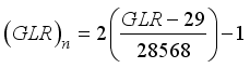 , for the clip scaling method.
  and
and  are adjusted to reflect the additional input parameters:
  ,
,  ,
,  and
and  . Using the appropriate weights and biases presented in Tables 8 and 9 for 5-input-based models and Tables 10 and 11 for 6-input-based models,
  and
and  would be established. The normalized additional input variables are expressed as
 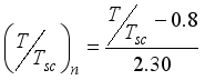 ,
,  ,
,  and
and 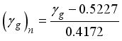 for the maximum-minimum normalization method and
  ,
,  ,
,  and
and  for the clip scaling method.
  ) estimations. The performance of (i.e., the closeness between) the models predicted
  with the actual field data was related using some statistical indices: coefficient of determination (R2), root mean square error (RMSE), average relative error (ARE) and average absolute relative error (AARE), and regression plot. The statistical indices are estimated using Equations 26 to 31:
  (26)
(26)  (27)
(27)  (28)
(28)  (29)
(29)  and
and  denote the field oil flow rate and average field flow rate, respectively,
  and
and  represent the predicted oil flow rate and average predicted oil flow rate, respectively, from the neural-based models, and
  denotes the number of datasets or data points.
  . The figure indicates that the neural and empirical correlations estimated data points aligned along the diagonal trend in Figure 11. According to Al-Bulushi et al.
  shows a good agreement between the predicted
  and the actual field
  datasets.
 Models | Statistical Performance | ||||
|---|---|---|---|---|---|
R2 | RMSE | ARE | AARE | ||
i. | Gilbert (1954) | 0.8717 | 1056.088 | -0.1268 | 0.3177 |
ii. | Baxendell (1958) | 0.9329 | 759.155 | 0.2513 | 0.3734 |
iii. | Ros (1960) | 0.9402 | 716.155 | 0.1688 | 0.3354 |
iv. | Achong (1961) | 0.8939 | 962.841 | 0.3927 | 0.4872 |
v. | Owolabi et al. (1991) | 0.9073 | 970.250 | 0.3358 | 0.5766 |
vi. | Beiranvand et al. (2012) | 0.9386 | 726.693 | -0.0264 | 0.3002 |
vii. | Okon et al. (2014) | 0.9627 | 877.850 | 0.4330 | 0.5187 |
viii. | Joshua et al. (2020) | 0.9477 | 669.982 | 0.0547 | 0.2998 |
ix. | ANN-MS | 0.9687 | 517.719 | 0.1012 | 0.2468 |
x. | ANN-CS | 0.9663 | 537.677 | 0.0673 | 0.2582 |
 with 98.67% and 97.20% for ANN-MS and ANN-CS models, respectively. Also, the RMSE, ARE, and AARE values obtained for the neural-based models were lesser than the empirical correlations’ estimations. Furthermore, the performance of the neural network-based models and the empirical correlations are in Figure 12. From the figure, the neural-based models and some correlations: Beiranvand et al.
  . The observation is visible in the data points (trend) for Khorzoughi et al.
 Models | Statistical Performance | ||||
|---|---|---|---|---|---|
R2 | RMSE | ARE | AARE | ||
i. | Beiranvand et al. [4] | 0.9468 | 718.010 | 0.1737 | 0.3300 |
ii. | Khorzoughi et al. [22] | 0.6560 | 2229.569 | 0.4601 | 0.7499 |
iii. | Okon et al. [23] | 0.9023 | 1253.268 | 0.5515 | 0.6486 |
iv. | Ghorbani et al [24] | 0.9255 | 926.690 | -0.1040 | 0.3742 |
v. | ANN-MS | 0.9867 | 383.276 | 0.1139 | 0.2367 |
vi. | ANN-CS | 0.9720 | 491.487 | 0.1144 | 0.2642 |
 than the empirical correlation estimations. Again, the error indicators (i.e., RMSE, ARE and AARE values) for the neural-based models were lesser than those obtained for the empirical correlations. Also, the neural models' predictions aligned diagonally more than the empirical correlations’ estimations in Figure 13. The observation implied that the neural-based models' predictions were in sync with the actual field datasets, with 98.08% and 97.91% certainty for the ANN-MS and ANN-CS models, respectively.
 Models | Statistical Performance | ||||
|---|---|---|---|---|---|
R2 | RMSE | ARE | AARE | ||
i. | Choubineh et al. [12] | 0.9443 | 721.958 | 0.0892 | 0.3316 |
ii. | Joshua et al. [26] | 0.9749 | 1089.123 | 0.3833 | 0.4196 |
iii. | ANN-MS | 0.9808 | 407.186 | 0.0643 | 0.2192 |
iv. | ANN-CS | 0.9791 | 424.931 | 0.0425 | 0.2594 |
Parameters | Data | Max. | Min. | Range | Mean | Std. Dev. | Kurt. | Coef. of Var. (%) |
|---|---|---|---|---|---|---|---|---|
Wellhead Pressure, | 63 | 2320.0 | 101.5 | 2218.6 | 592.93 | 445.31 | 2.957 | 75.10 |
Bean (Choke) Size, | 63 | 72.0 | 16.0 | 56.0 | 35.46 | 13.96 | 0.268 | 39.38 |
Gas-Liquid Ratio, | 63 | 4134.41 | 93.26 | 4041.15 | 889.64 | 925.15 | 4.802 | 103.99 |
Parameters | Data | Max. | Min. | Range | Mean | Std. Dev. | Kurt. | Coef. of Var. (%) |
|---|---|---|---|---|---|---|---|---|
Wellhead Pressure, | 113 | 2940.0 | 50.0 | 2890.0 | 1280.1 | 348.69 | 1.275 | 77.13 |
Bean (Choke) Size, | 113 | 80.0 | 24.0 | 56.0 | 54.51 | 16.88 | 0.122 | 43.89 |
Gas-Liquid Ratio, | 113 | 3660.0 | 107.0 | 3553.0 | 858.58 | 440.25 | 8.518 | 206.33 |
Oil Gravity, | 113 | 0.92 | 0.808 | 0.112 | 0.8583 | 0.0171 | -0.047 | 5.30 |
Temperature, | 113 | 135.0 | 90.0 | 45.0 | 124.12 | 12.61 | 0.384 | 29.81 |
Gas Gravity, | 113 | 1.236 | 0.6886 | 0.5474 | 0.7313 | 0.0597 | -0.805 | 3.14 |
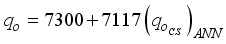
 resulted in R2 values of 0.9488 for ANN-MS, while the ANN-CS model had 0.9644. From a statistical standpoint, the R2 values implied that the simplified neural-based models predicted
  are 94.88% (for ANN-MS) and 96.44% (for ANN-CS) related to the Okon et al.
  datasets with 88.48% and 92.64% certainty for ANN-MS and ANN-CS models, respectively. Aside from the R2 values that depict the predicted
  ’s closeness with the test datasets, the generality robustness of these simplified neural-based models is visible on the cross-plots in Figures 14 to 17. As observed in these figures, the diagonal trend of the data points indicates a good agreement between the predicted
  and the test datasets
 Datasets Source | Neural Model | Statistical Performance | ||||
|---|---|---|---|---|---|---|
R2 | RMSE | ARE | AARE | |||
i. | Okon et al. [23] | ANN-MS | 0.9488 | 251.926 | 0.1158 | 0.1862 |
ANN-CS | 0.9644 | 205.781 | 0.0248 | 0.1275 | ||
ii. | Choubineh et al. [12] | ANN-MS | 0.8848 | 2754.48 | 0.0746 | 0.2573 |
ANN-CS | 0.9264 | 2089.93 | 0.1656 | 0.2267 | ||
 data with 89.08% certainty for ANN-MS and 92.64% for ANN-CS. Also, the closeness of the model’s predictions with the test datasets is visible on the diagonal alignment of the predicted
  and test datasets in the cross-plots (Figures 18 and 19). Thus, the generalization performance of the simplified neural-based models is about 90.0% certainty with the test datasets.
 Datasets Source | Neural Model | Statistical Performance | ||||
|---|---|---|---|---|---|---|
R2 | RMSE | ARE | AARE | |||
i. | Choubineh et al. [12] | ANN-MS | 0.8908 | 2655.50 | 0.1484 | 0.2219 |
ANN-CS | 0.9264 | 2089.93 | 0.1656 | 0.2267 | ||
 values were closer to the actual test datasets than the estimated
  from the empirical correlations. The neural-based models’ predictions for the Choubineh et al.
  from the empirical correlations as the R-values obtained for these models were close. On the other hand, the simplified 6-input-based neural models’ generalization performance was comparable with the correlations of Choubineh et al.
 Models | Statistical Performance | ||||||||
|---|---|---|---|---|---|---|---|---|---|
Okon et al. (2015). Datasets | Choubineh et al. (2017) Datasets | ||||||||
R2 | RMSE | ARE | AARE | R2 | RMSE | ARE | AARE | ||
i. | Gilbert [14] | 0.5099 | 944.51 | -0.4403 | 0.3349 | 0.8117 | 2451.04 | 0.1957 | -0.1924 |
ii. | Baxendell [15] | 0.5062 | 1120.79 | 0.0504 | 0.3254 | 0.9596 | 1130.74 | -0.0110 | 0.0904 |
iii. | Ros [16] | 0.5070 | 1111.48 | -0.0093 | 0.3182 | 0.9548 | 1138.66 | 0.0261 | 0.0941 |
iv. | Achong [17] | 0.4805 | 1218.12 | 0.1445 | 0.3665 | 0.9555 | 1128.76 | 0.0161 | 0.0989 |
v. | Pilehvari [19] | 0.4977 | 2971.07 | 0.8235 | 0.8828 | 0.9394 | 10379.76 | 0.9623 | 0.9623 |
vi. | Beiranvand et al. [4] | 0.4574 | 1210.70 | -0.1398 | 0.3833 | 0.9495 | 1205.77 | 0.0868 | 0.1339 |
vii. | Okon et al. [23] | 0.5319 | 1053.51 | 0.1658 | 0.3660 | 0.9345 | 1371.86 | 0.0157 | 0.1154 |
viii. | Owolabi et al. [ 20] | 0.5210 | 1059.91 | 0.0323 | 0.3461 | 0.9302 | 141620 | -0.0023 | 0.1184 |
ix. | Joshua et al. [26] | 0.4821 | 1246.46 | -0.0756 | 0.3469 | 0.9334 | 1383.10 | -0.0010 | 0.1234 |
x. | ANN-MS | 0.9488 | 251.926 | 0.1158 | 0.1862 | 0.8848 | 2754.48 | 0.0746 | 0.2573 |
xi. | ANN-CS | 0.9644 | 205.781 | 0.0248 | 0.1275 | 0.9264 | 2089.93 | 0.1656 | 0.2267 |
Models | Statistical Performance | ||||
|---|---|---|---|---|---|
R2 | RMSE | ARE | AARE | ||
i. | Choubineh et al. [12] | 0.9695 | 1077.45 | -0.0089 | 0.0941 |
ii. | Joshua et al. [26] | 0.8949 | 1786.34 | 0.2262 | 0.2450 |
iii. | ANN-MS | 0.8908 | 2655.50 | 0.1484 | 0.2219 |
iv. | ANN-CS | 0.9264 | 2089.93 | 0.1656 | 0.2267 |
 ), a non-parametric method alternative to the one-way analysis of variance (ANOVA), was evaluated using Equation 30 to test whether the models’ predicted and field test oil flow rate datasets have the same mean values. Therefore, the null hypothesis (*H0) is whether a significant difference exists between predicted models and the field oil flow rate mean values.
  (30)
(30)  is the H-test value, which is equivalent to the critical value of Chi-square (
  ),
),  represents the total number of data points in the test,
  denotes the number of data groups in the test,
  is the rank sum of the individual group in the test and
  is the number of data points in each group.
  values obtained, which are equivalent to the critical values of Chi-square (
  ). Based on the critical values table, at 2 degrees of freedom, the corresponding p-values visible in Table 22 for the
  values are less than the p-value of 0.05. Therefore, the null hypothesis (*H0) that no significant difference exists between the models predicted and field test oil flow rate mean values are accepted. Hence, the developed models (ANN-MS and ANN-CS) predictions of oil flow rate are statistically significant and acceptable.
 Datasets source |
| p-values | Null hypothesis (*H0) | |
|---|---|---|---|---|
i. | Field test | 6.6721 | 0.0377 | Accept |
ii. | Okon et al. [23] | 6.5562 | 0.0398 | Accept |
iii. | Choubineh et al. [12] | 7.6463 | 0.0478 | Accept |
 ) than basic sediments and water (BS&W) and gas gravity (γg); and
 AARE | Average Absolute Relative Error |
AI | Artificial Intelligence |
ANN | Artificial Neural Network |
ANN-CS | Clip Scaling Trained ANN |
ANN-MS | Maximum-Minimum Scaling trained ANN |
ARE | Average Relative Error |
At | Tubing Cross-Section Area |
BHP | Bottomhole Pressure |
BHT | Bottomhole Temperature |
BS&W | Basic Sediment & Water |
CF | Contribution Factor |
CNN | Convolution Neural Network |
DNN | Deep Neural Network |
Coef. of Var. | Coefficient of Variance |
| Open Hole Size |
FBHP | Flowing Bottomhole Pressure |
FFBP | Feed-Forward Back-Propagation |
GLR | Gas-Liquid Ratio |
GOR | Gas-Oil Ratio |
H | Well Depth |
H-test | Kruskal-Wallis Test |
k | Permeability |
Kurt. | Kurtosis |
Le | Effective Length |
MAPE | Mean Absolute Percentage Error |
MISO | Multiple-Inputs Single-Output |
ML | Machine Learning |
MLP | Multilayer Perceptron |
MSE | Mean Square Error |
| Number of Laterals |
| Flowline Pressure |
| Gas lift Pressure |
| Reservoir Pressure |
| Wellhead Pressure |
| Critical Liquid flow Rate |
| Gas Lift Rate |
| Liquid Flow Rate |
| Oil Flow Rate |
| Critical Oil flow Rate |
R | Correlation Coefficient |
R2 | Coefficient of Determination |
RF | Random Forest |
RBF | Radial Basis Function |
RI | Relative Importance |
RMSE | Root Mean Square Error |
RNN | Recurrent Neural Network |
S | Choke (Bean) Size |
T | Temperature |
THP | Tubing Head Pressure |
Tsc | Temperature at Surface Condition |
WHT | Wellhead Temperature |
WCT | Water-Cut |
| Chi-Square |
| Gas Gravity |
| Oil Gravity |
| [1] | Bikmukhametov T, Jäschke J (2020) First principles and machine learning virtual flow metering: A literature review. J Pet Sci Eng, 184: 106487-106592. |
| [2] | Al-Jawad MS, Ottba DJS (2006) Well performance analysis based on flow calculations and IPR. J Eng, 13(3): 822-841. |
| [3] | Agwu OE, Alkouh A, Alatefi S, Azim RA, Ferhadi R (2024) Utilization of machine learning for the estimation of production rates in wells operated by electrical submersible pumps. J Pet Explor Prod Technol, 14: 1205–1233. |
| [4] | Beiranvand MS, Mohammadmoradi P, Aminshahidy B, Fazelabdolabadi B, Aghahoseini S (2012) New multiphase choke correlations for a high flow rate Iranian Oil Field. J Mech Sci, 3: 43-47. |
| [5] | Okon AN, Appah D (2018) Water coning prediction: An evaluation of horizontal well correlations. Eng and Applied Sci J, 3(1): 21-28. |
| [6] |
Ejoh E (2017) How Nigeria ‘lost N2 trillion to poor metering of oil wells’ in two years. Vanguard Online.
https://www.vanguardngr.com/2017/05/nigeria-lost-n2-trillion-poor-metering-oil-wells-two-years/ |
| [7] | Brill JP (2010) Modeling multiphase flow in pipes. Soc Pet Eng.: The Way Ahead, 6(2): 16-17. |
| [8] | Lak A, Azin R, Osfouri S, Fatehi R (2017) Modelling critical flow through choke for a gas-condensate reservoir based on drill stem test data. Iranian J Oil & Gas Sci and Technol, 6(3): 29-40. |
| [9] | Nasriani HR, Kalantariasl A (2011) Two-phase flow choke performance in high-rate gas condensate wells. Paper presented at the Society of Petroleum Engineers Asia Pacific Oil and Gas Conference and Exhibition, Jakarta, Indonesia, 20-22 Sept. 2011. |
| [10] | Hong KC, Griston S (1997) Best practice for the distribution and metering of two-phase steam. Soc Pet Eng. Production Facility, 12(3): 173-80. |
| [11] | Sadatshojaei E, Jamialahmadi M, Esmaeilzadeh F, Ghazanfari MH (2016) Effects of low-salinity water coupled with silica nanoparticles on wettability alteration of dolomite at reservoir temperature. J Pet Sci Technol, 34(15): 1345-1351. |
| [12] | Choubineh A, Ghorbani H, Wood DA, Moosavi SR, Khalafi E, Sadatshojaei E (2017) Improved predictions of wellhead choke liquid critical-flow rates: Modelling based on hybrid neural network training learning-based optimization. Fuel, 207: 547-560. |
| [13] | Al-Attar HH (2009) New correlations for critical and subcritical two-phase flow through surface chokes in high-rate oil wells. Paper presented at the Latin American and Caribbean Petroleum Engineering Conference, Cartagena de Indias, Colombia, 31 May-30 June 2009. |
| [14] | Gilbert WE (1954) Flowing and gas-lift well performance. American Petroleum Institute Drilling & Production Practice, Dallas, Texas, 20: 126-157. |
| [15] | Baxendell PB (1957) Bean Performance-Lake Wells. Shell Internal Report, October 1957. |
| [16] | Ros NCJ (1960) An analysis of critical simultaneous gas/liquid flow through a restriction and its application to flow metering. Applied Sci Res, 9: 374-389. |
| [17] | Achong I (1961) Revised bean performance formula for Lake Maracaibo wells. Shell Internal Report, Oct. 1961. |
| [18] | Omana R, Houssier C, Brown KE, Brill JP, Thompson RE (1968) Multiphase flow through chokes. Paper presented at the Society of Petroleum Engineers Annual Meeting, Denver Colorado, 28 Sept. - 1 Oct. 1968. |
| [19] | Pilehvari AA (1981) Experimental study of critical two-phase flow through wellhead chokes. University of Tulsa Fluid Flow Project Report, Tulsa, USA. |
| [20] | Owolabi OO, Dune KK, Ajienka JA (1991) Producing the multiphase flow performance through wellhead chokes for the Niger Delta oil wells. Paper presented at the International Conference of the Society of Petroleum Engineers Nigeria Section Annual Proceeding, August 1991. |
| [21] | Al-Towailib A, Al-Marhoun MA (1994) A new correlation for two-phase flow through chokes. J Can Pet Technol, 33(5): 40-43. |
| [22] | Khorzoughi MB, Beiranvand M, Rasaei MR (2013) Investigation of a new multiphase flow choke correlation by linear and non-linear optimization methods and Monte Carlo sampling. J Pet Explor Prod Technol, 3: 279-285. |
| [23] | Okon AN, Udoh FD, Appah D (2015) Empirical wellhead pressure production rate correlations for Niger Delta oil wells. Paper presented at the Society of Petroleum Engineers (SPE), Nigeria Council 39th Nigeria Annual International Conference and Exhibition, Eko Hotel and Suite, Lagos, 4-6 Aug. 2015. |
| [24] | Ghorbani H, Wood DA, Choubineh A, Tatar A, Abarghoy PG, Madani M, Mohamadian N (2018) Prediction of oil flow rate through an orifice flow meter: artificial intelligence alternatives compared. Petroleum 6 (4): 404-414. |
| [25] | Alrumah M, Alenezi RA (2019) New universal two-phase choke correlations developed using non-linear multivariable optimization technique. J Eng Res, 7(3): 320-329. |
| [26] | Joshua SK, Oshokosikeshishi LP, Sylvester O (2020) New production rate model of wellhead choke for Niger Delta oil wells. J Pet Sci Tech, 10: 41-49. |
| [27] | Alarifi SA (2022). Workflow to predict wellhead choke performance during multiphase flow using machine learning. J Pet Sci Eng, 214 (2022)110563. |
| [28] | Berneti SM, Shahbazian M (2011) An imperialist competitive algorithm artificial neural network method to predict oil flow rate of the wells. Int. J. Comput. Appl. 26(10): 47-50. |
| [29] | Mirzaei-Paiaman A, Salavati S (2012) The application of artificial neural networks for the prediction of oil production flow rate. Energy Sources, Part A: Recovery, Utilization, and Environmental Effects, 34(19): 1834-1843. |
| [30] | Al-Khalifa MA, Al-Marhoun MA (2013) Application of neural network for two-phase flow through chokes. Paper presented at the Society of Petroleum Engineers Saudi Arabia section Annual Technical Symposium and Exhibition, Khobar, Saudi Arabia, 19-22 May 2013. |
| [31] | Zangl G, Hermann R, Schweiger C (2014) Comparison of methods for stochastic multiphase flow rate estimation. Paper presented at the Society of Petroleum Engineers Annual Technical Conference and Exhibition, Amsterdam, The Netherlands, 27-29 Oct. 2014. |
| [32] | Al-Ajmi MD, Alarifi SA, Mahsoon AH (2015) Improving multiphase choke performance prediction and well production test validation using artificial intelligence: A new milestone. Paper presented at the Society of Petroleum Engineers Digital Energy Conference and Exhibition, Woodlands, Texas, USA, 3-5 Mar. 2015. |
| [33] | Okon AN, Appah D (2016) Neural network models for predicting wellhead pressure-flow rate relationship for Niger Delta oil wells. J Scientific Res Reports, 12(1): 1-14. |
| [34] | Al-Qutami TA, Ibrahim R, Ismail I, Ishak MA (2018) Virtual multiphase flow metering using diverse neural network ensemble and adaptive simulated annealing. Expert Syst. Appl. 93(1): 72-85. |
| [35] | Al-Kadem M, Al Dabbous M, Al Mashhad A, Al Sadah H (2019) Utilization of artificial neural networking for real-time oil production rate estimation. Paper presented at the Abu Dhabi International Petroleum Exhibition and Conference, Abu Dhabi, UAE, 11-14 Nov. 2019. |
| [36] | Khan MR, Tariq Z, Abdulraheem A (2020) Application of artificial intelligence to estimate oil flow rate in gas-lift wells. Natural Resources Research, 29: 4017-4029. |
| [37] | Ibrahim NM, Alharbi AA, Alzahrani TA, Abdulkarim AM, Alessa IA, Hameed AM, Albabtain AS, Alqahtani DA, Alsawwaf MK, Almuqhim AA (2022) Well performance classification and prediction: deep learning and machine learning long term regression experiments on oil, gas, and water production. Sensors, 22, 5326. |
| [38] | Okorugbo O, Dune KK, Wami EN (2021) Application of neural network-particle swarm modelling for predicting wellhead choke performance in the Niger Delta. Int J Pet Petrochem Eng, 7(1): 21-29. |
| [39] | Park YS, Lek S (2016) Artificial neural networks: multilayer perceptron for ecological modelling. In S. E. Jørgensen (Ed.), Developments in environmental modelling, 28: 123-140). Elsevier. |
| [40] | Behnoud P, Hosseini P (2017) Estimation of lost circulation amount occurs during under balanced drilling using drilling data and neural network. Egyptian J Pet, 26(3): 627-634. |
| [41] | Mekanik F, Imteaz M, Gato-Trinidad S, Elmahdi A (2013) Multiple regression and artificial neural network for long term rainfall forecasting using large scale climate modes. J. Hydrol, 503(2): 11-21. |
| [42] | Demuth, H., Beale, M., Martin, H. (2009). Neural network toolbox users guide. The Mathworks, Inc, p. 906, Version 6. |
| [43] | Haykin S (1999) Neural networks, a comprehensive foundation, Second ed. Prentice Hall Inc., Upper Saddle River. |
| [44] | Aalst WMP, Rubin V, Verbeek HMW, Van Dongen BF, Kindler E, Günther CW (2010) Process mining: a two-step approach to balance between underfitting and overfitting. Software Syst. Model, 9(1): 87-111. |
| [45] | Anifowose F, Ewenla A, Eludiora S (2012) Prediction of oil and gas reservoir properties using support vector machines. Paper presented at the International Petroleum Technical Conference, Bangkok, Thailand, 7-9 Feb. 2012. |
| [46] | Okon AN, Ansa IB (2021) Artificial neural network models for reservoir aquifer dimensionless variables: influx and pressure prediction for water influx calculation. J Pet Explor Prod Technol, 11(4): 1885-1904. |
| [47] | Perkins TK (1993) Critical and subcritical flow of multiphase mixtures through chokes. Society of Petroleum Engineering Drilling and Completion, 8(4): 271-276. |
| [48] | Ibrahim AF, Al-Dhaif R, Elkatatny S, Al Shehri D (2021) Applications of artificial intelligence to predict oil rate for high gas-oil ratio and water-cut wells. ACS Omega, 6: 19484-19493. |
| [49] | Barjouei HS, Ghorbani H, Mohamadian N, Wood DA, Davoodi S, Moghadasi J, Saberi H (2021) Prediction performance advantages of deep machine learning algorithms for two‑phase flow rates through wellhead chokes. J Pet Explor Prod, 11: 1233–1261. |
| [50] | Ahmadi MA, Ebadi M, Shokrollahi A, Majidic SMJ (2013) Evolving artificial neural network and imperialist competitive algorithm for prediction oil flow rate of the reservoir. Appl. Soft Comput. 13 (2), 1085-1098. |
| [51] | Gorjaei RG, Songolzadeh R, Torkaman M, Safari M, Zargar G (2015) A novel PSO-LSSVM model for predicting liquid rate of two-phase flow through wellhead chokes. J Nat Gas Sci Eng, 24: 228-237. |
| [52] | Hasanvand M, Berneti SM (2015) Predicting oil flow rate due to multiphase flow meter by using an artificial neural network. Energy Sources, Part A: Recovery, Utilization, and Environmental Effects, 37(8): 840-845. |
| [53] | Baghban A, Abbasi P, Rostami P, Bahadori M, Ahmad Z, Kashiwao T, Bahadori A (2016) Estimation of oil and gas properties in petroleum production and processing operations using rigorous model. J Pet Sci Tech, 34(13): 1129-1136. |
| [54] | Buhulaigah A, Al-Mashhad AS, Al-Arifi SA, Al-Kadem MS, Al-Dabbous MS (2017) Multilateral wells evaluation utilizing artificial intelligence. Paper presented at the Society of Petroleum Engineers Middle East Oil & Gas Show and Conference, Manama, Kingdom of Bahrain, 6-9 Mar. 2017. |
| [55] | Khan MR, Alnuaim S, Tari Z, Abdulraheem A (2019) Machine learning application for oil rate prediction in artificial gas lift wells. Paper presented at the Society of Petroleum Engineers Middle East Oil and Gas Show and Conference, Manama, Bahrain, 18-21 Mar. 2019. |
| [56] | Ghorbani H, Wood, DA, Moghadasi J, Choubineh A, Abdizadeh P, Mohamadian, N (2019) Predicting liquid flow-rate performance through wellhead chokes with genetic and solver optimizers: an oil field case study. J Pet Explor Prod Technol, 9: 1355-1373. |
| [57] | Al-Rumah M, Aladwani F, Alatefi S (2020) Toward the development of a universal choke correlation - global optimization and rigorous computational techniques. J Eng Res, 8(3): 240-254. |
| [58] | Marfo SA, Kporxah C (2020) Predicting oil production rate using artificial neural network and decline curve analytical methods. Proceedings of 6th UMaT Biennial International Mining and Mineral Conference, Tarkwa, Ghana, 43-50. |
| [59] | Azim RA (2022) A new correlation for calculating wellhead oil flow rate using artificial neural network. J Artificial Intelligence in Geosciences, 3: 1-7. |
| [60] | Okon AN, Effiong AJ, Daniel DD (2023) Explicit neural network-based models for bubble point pressure and oil formation volume factor prediction. Arabian J Sci Eng, 48: 9221-9257. |
| [61] | Mahmoudi S, Mahmoudi A (2014) Water saturation and porosity prediction using back-propagation artificial neural network (BPANN) from well log data. J Eng & Technol 5(2): 1-8. |
| [62] | Okon AN, Adewole SE, Uguma EM (2020) Artificial neural network model for reservoir petrophysical properties: porosity, permeability and water saturation prediction. J Model Earth Syst and Environ, 7: 2373-2390. |
| [63] | Abuh FA, Akpabio JU, Okon AN (2023) Machine learning-based models for basic sediment & water and sand-cut prediction in matured Niger Delta fields. J Energy Res Reviews 15(2): 70-93. |
| [64] | Al-Bulushi N, King PR, Blunt MJ, Kraaijveld M (2009) Development of artificial neural network models for predicting water saturation and fluid distribution. J Pet Sci Eng 68: 197-208. |
| [65] | Sircar A, Yadav K, Rayavarapu K, Bist N, Oza H (2021) Application of machine learning and artificial intelligence in oil and industry. Pet Res, 6: 379-391. |
| [66] | Effiong AJ, Etim JO, Okon AN (2021) Artificial intelligence model for predicting formation damage in oil and gas wells. Paper presented at the Society of Petroleum Engineers (SPE), Nigeria Council 45th Nigeria Annual International Conference and Exhibition, 2-4 Aug. 2021. |
| [67] | George A (2021) Predicting oil production flow rate using artificial neural networks – the Volve field case. Paper presented at the Nigeria Annual International Conference and Exhibition, Logas, Nigeria, 2-4 August 2021. |
| [68] | Citakoglu H, Coskun O (2022) Comparison of hybrid machine learning methods for the prediction of short-term meteorological droughts of Sakarga Meterological Station in Turkey. Environ Sci Poll Res. |
| [69] | Demir V (2022) Enhancing monthly lake levels forecasting using heuristic regression techniques with periodicity data component: application of Lake Michigan. Theor Appl Climatol 148: 915-929. |
| [70] | Alexander D, Tropsha A, Winkler D (2015) Beware of R2: simple, unambiguous assessment of the prediction accuracy of QSAR and QSPR Models. J Chem Info Model, 55(7): 1316-1322. |
APA Style
Umana, U. K., Okon, A. N., Agwu, O. E. (2024). Simplified Neural Network-Based Models for Oil Flow Rate Prediction. Petroleum Science and Engineering, 8(2), 70-99. https://doi.org/10.11648/j.pse.20240802.12
ACS Style
Umana, U. K.; Okon, A. N.; Agwu, O. E. Simplified Neural Network-Based Models for Oil Flow Rate Prediction. Pet. Sci. Eng. 2024, 8(2), 70-99. doi: 10.11648/j.pse.20240802.12
AMA Style
Umana UK, Okon AN, Agwu OE. Simplified Neural Network-Based Models for Oil Flow Rate Prediction. Pet Sci Eng. 2024;8(2):70-99. doi: 10.11648/j.pse.20240802.12
@article{10.11648/j.pse.20240802.12,
  author = {Uduak Koffi Umana and Anietie Ndarake Okon and Okorie Ekwe Agwu},
  title = {Simplified Neural Network-Based Models for Oil Flow Rate Prediction
},
  journal = {Petroleum Science and Engineering},
  volume = {8},
  number = {2},
  pages = {70-99},
  doi = {10.11648/j.pse.20240802.12},
  url = {https://doi.org/10.11648/j.pse.20240802.12},
  eprint = {https://article.sciencepublishinggroup.com/pdf/10.11648.j.pse.20240802.12},
  abstract = {Available neural network-based models for predicting the oil flow rate (qo) in the Niger Delta are not simplified and are developed from limited data sources. The reproducibility of these models is not feasible as the models’ details are not published. This study developed simplified and reproducible three, five, and six-input variables neural-based models for estimating qo using 283 datasets from 21 wells across fields in the Niger Delta. The neural-based models were developed using maximum-minimum (max.-min.) normalized and clip-normalized datasets. The performances and the generalizability of the developed models with published datasets were determined using some statistical indices: coefficient of determination (R2), mean square error (MSE), root mean square error (RMSE), average relative error (ARE) and average absolute relative error (AARE). The results indicate that the 3-input-based neural models had overall R2, MSE, and RMSE values of 0.9689, 9.6185x10⁻⁴ and 0.0310, respectively, for the max.-min. normalizing method and R2 of 0.9663, MSE of 5.7986x10⁻³ and RMSE of 0.0762 for the clip scaling approach. The 5-input-based models resulted in R2 of 0.9865, MSE of 5.7790×10⁻⁴ and RMSE of 0.0240 for the max.-min. scaling method and R2 of 0.9720, MSE of 3.7243x10⁻³ and RMSE of 0.0610 for the clip scaling approach. Also, the 6-input-based models had R2 of 0.9809, MSE of 8.7520x10⁻⁴ and RMSE of 0.0296 for the max.-min. normalizing approach and R2 of 0.9791, MSE of 3.8859 x 10⁻³ and RMSE of 0.0623 for the clip scaling method. Furthermore, the generality performance of the simplified neural-based models resulted in R2, RMSE, ARE, and AAPRE of 0.9644, 205.78, 0.0248, and 0.1275, respectively, for the 3-input-based neural model and R2 of 0.9264, RMSE of 2089.93, ARE of 0.1656 and AARE of 0.2267 for the 6-input-based neural model. The neural-based models predicted qo were more comparable to the test datasets than some existing correlations, as the predicted qo result was the lowest error indices. Besides, the overall relative importance of the neural-based models’ input variables on qo prediction is S>GLR>Pwh>T/Tsc>γo>BS&W>γg. The simplified neural-based models performed better than some empirical correlations from the assessment indicators. Therefore, the models should apply as tools for oil flow rate prediction in the Niger Delta fields, as the necessary details to implement the models are made visible.
},
 year = {2024}
}
TY  - JOUR
T1  - Simplified Neural Network-Based Models for Oil Flow Rate Prediction

AU  - Uduak Koffi Umana
AU  - Anietie Ndarake Okon
AU  - Okorie Ekwe Agwu
Y1  - 2024/09/23
PY  - 2024
N1  - https://doi.org/10.11648/j.pse.20240802.12
DO  - 10.11648/j.pse.20240802.12
T2  - Petroleum Science and Engineering
JF  - Petroleum Science and Engineering
JO  - Petroleum Science and Engineering
SP  - 70
EP  - 99
PB  - Science Publishing Group
SN  - 2640-4516
UR  - https://doi.org/10.11648/j.pse.20240802.12
AB  - Available neural network-based models for predicting the oil flow rate (qo) in the Niger Delta are not simplified and are developed from limited data sources. The reproducibility of these models is not feasible as the models’ details are not published. This study developed simplified and reproducible three, five, and six-input variables neural-based models for estimating qo using 283 datasets from 21 wells across fields in the Niger Delta. The neural-based models were developed using maximum-minimum (max.-min.) normalized and clip-normalized datasets. The performances and the generalizability of the developed models with published datasets were determined using some statistical indices: coefficient of determination (R2), mean square error (MSE), root mean square error (RMSE), average relative error (ARE) and average absolute relative error (AARE). The results indicate that the 3-input-based neural models had overall R2, MSE, and RMSE values of 0.9689, 9.6185x10⁻⁴ and 0.0310, respectively, for the max.-min. normalizing method and R2 of 0.9663, MSE of 5.7986x10⁻³ and RMSE of 0.0762 for the clip scaling approach. The 5-input-based models resulted in R2 of 0.9865, MSE of 5.7790×10⁻⁴ and RMSE of 0.0240 for the max.-min. scaling method and R2 of 0.9720, MSE of 3.7243x10⁻³ and RMSE of 0.0610 for the clip scaling approach. Also, the 6-input-based models had R2 of 0.9809, MSE of 8.7520x10⁻⁴ and RMSE of 0.0296 for the max.-min. normalizing approach and R2 of 0.9791, MSE of 3.8859 x 10⁻³ and RMSE of 0.0623 for the clip scaling method. Furthermore, the generality performance of the simplified neural-based models resulted in R2, RMSE, ARE, and AAPRE of 0.9644, 205.78, 0.0248, and 0.1275, respectively, for the 3-input-based neural model and R2 of 0.9264, RMSE of 2089.93, ARE of 0.1656 and AARE of 0.2267 for the 6-input-based neural model. The neural-based models predicted qo were more comparable to the test datasets than some existing correlations, as the predicted qo result was the lowest error indices. Besides, the overall relative importance of the neural-based models’ input variables on qo prediction is S>GLR>Pwh>T/Tsc>γo>BS&W>γg. The simplified neural-based models performed better than some empirical correlations from the assessment indicators. Therefore, the models should apply as tools for oil flow rate prediction in the Niger Delta fields, as the necessary details to implement the models are made visible.

VL  - 8
IS  - 2
ER  -
Department of Petroleum Engineering, University of Uyo, Uyo, Nigeria
Department of Petroleum Engineering, University of Uyo, Uyo, Nigeria
Department of Petroleum Engineering, University of Uyo, Uyo, Nigeria
Figure 1. A simple representation of oil and gas production system [2].
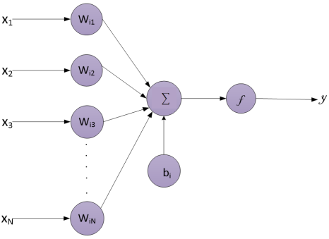
Figure 2. A typical ANN architecture [45, 46].
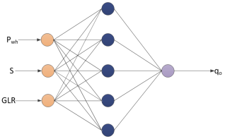
Figure 3. Neural network architecture for a 3-input-based model.
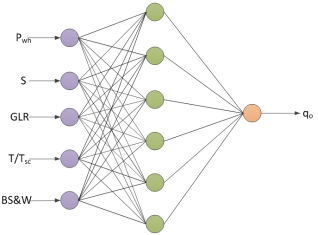
Figure 4. Neural network architecture for a 5-input-based model.
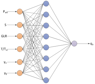
Figure 5. Neural network architecture for a 6-input-based model.
Figure 6. Flowchart of the processes involved in performing the study.
Figure 7. Comparison of the normalization approaches overall performance for the 3-input-based network.
Figure 8. Comparison of the normalization approaches overall performance for the 5-input-based network.
Figure 9. Comparison of the normalization approaches overall performance for the 6-input-based network.
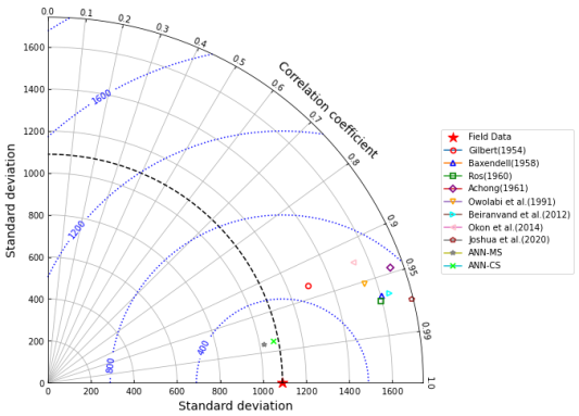
Figure 10. Taylor diagram of the 3-input-based models with some empirical correlations.
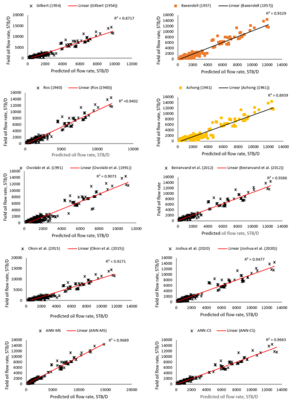
Figure 11. Comparison of the 3-input-based neural models and empirical correlations predictions; the diagonal line represents 1:1 trend line.
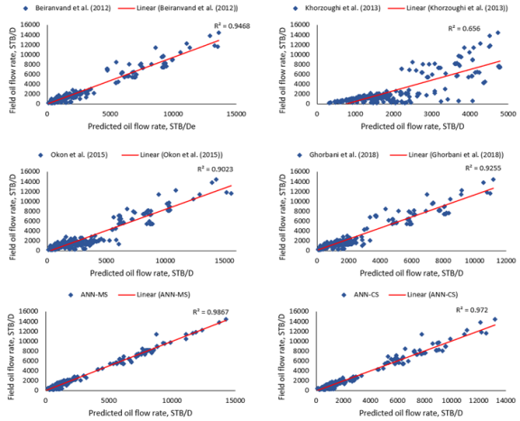
Figure 12. Comparison of the 5-input-based neural models and empirical correlations predictions; the diagonal line represents 1:1 trend line.
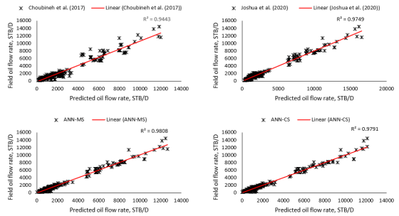
Figure 13. Comparison of the 6-input-based neural models and empirical correlations predictions; the diagonal line represents 1:1 trend line.
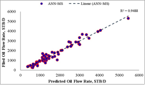
Figure 14. Comparison of 3-input-based model (ANN-MS) predictions with oil flow rate datasets from Okon et al. [23].
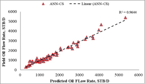
Figure 15. Comparison of 3-input-based model (ANN-CS) predictions with oil flow rate datasets from Okon et al. [23].

Figure 16. Comparison of 3-input-based model (ANN-MS) predictions with oil flow rate datasets from Choubineh et al. [12].
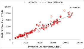
Figure 17. Comparison of 3-input-based model (ANN-CS) predictions with oil flow rate datasets from Choubineh et al. [12].
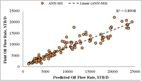
Figure 18. Comparison of 6-input-based model (ANN-MS) predictions with oil flow rate datasets from Choubineh et al. [12].
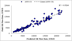
Figure 19. Comparison of 6-input-based model (ANN-CS) predictions with oil flow rate datasets from Choubineh et al. [12].


 ,
, 

 ,
,  ,
, 

 , k,
, k,  ,
, 


 , THP, FBHP, t


 )
)
 )
)
 )
)


 )
)
 )
)
 )
) )
)
 values
